Introduction to spectral processing
What does ‘spectral’ processing mean? There is a wide range of concepts that are linked to this word, but they all point to manipulating the components of a sound waveform, and the principle of breaking down an audio signal into a set of such components. So, from this perspective, any audio signal is made up of simpler, pure, sound waveforms, which, combined, provide us with the various sounds we hear. It is an idea that goes back to Helmholtz’s pioneer studies in the nineteenth century, which applied to sound waves the mathematical principles outlined earlier on by Fourier. The simple, pure, components in this analysis are sinusoidal (sine, cosine) waves. We can call the set of such waves, which, combined, make up an audio signal, the spectrum of that sound.

The Fourier Transform
In order to obtain the ‘recipe’ for a given ‘mix’ of sinusoids that will reproduce a target sound, we can apply a number of analytical methods, many of which are based on a single principle, the Fourier Transform (FT). What we will try to find out is this: given a sound we want to reproduce, what are its sinusoidal components?

These components will be identified by three parameters: frequency, amplitude and phase. The first is related to how high or how low the component is (think, in a very loose way, of pitch); and the second, how prevalent it is in the mix (how much energy it has, relatively). The third is more subtle: it indicates whether the component is either a sine, a cosine, an inverted sine, an inverted cosine, or something in between this four shapes. The difference between a sine and a cosine wave is that the latter starts a quarter cycle later than the former. Inverted forms of these are half-cycle delayed in relation to the original waves. So we can see then that phase has to do with the synchronisation (time delay) between the start positions of the various components.

So, how does it work? Well, the idea is straightforward, although its mathematical formulation might be seen as complicated. The FT uses a pair of sinusoid functions (a cosine and a sine), which make up what we call a complex sinusoid, as a component ‘detector’. Such detectors are placed at all possible frequencies from –infinity to +infinity, and at each frequency the FT multiplies the signal being analysed (which is taken to extend from –infinity to +infinity in time) with the respective sinusoid. This multiplication is point-by-point (every infinitesimal value of each signal) and the results at all of these points are then added together (an integral sum). The FT output is then the amplitude of cosines and sines detected in each frequency, called a spectral coefficient. If there is no component at that given frequency, this amplitude is zero and nothing is detected.

So this gives us all the data we need: frequency of the component (which is the frequency of the ‘detector’ sinusoid), its amplitude (spread out in the sine and cosine parts, obtained from the magnitude of the coefficient) and the phase (which can be worked out from the balance of energy in the sine and cosine parts, or the argument of coefficient). There is only a little snag. The FT cannot be implemented in a digital computer. It is based on continuous time and continuous frequency (Steiglitz 1994), which is not really suited to such an implementation. It remains a useful mathematical tool, however.

The Discrete Fourier Transform
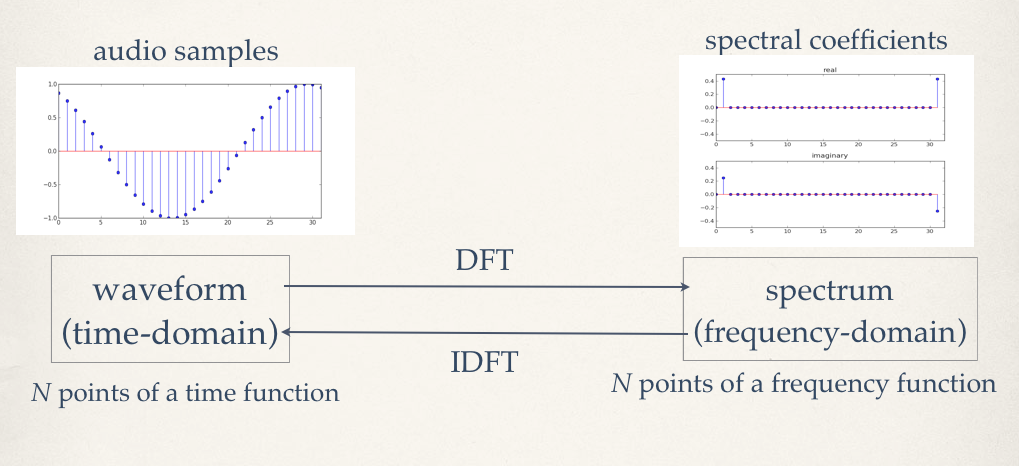
What we need is a discrete form of this operation. A formulation of the transform that is adapted to sampled signals: the Discrete Fourier Transform. From the original FT, we keep the basic method, we will use a complex sinusoid as a detector. Now, instead of using sinusoids at all possible frequencies, we will set these in a grid at discrete steps. The input signal will also be time constrained, a window of a given duration will be used. Finally, the output will also be constrained, just a set of amplitudes for cosines and sines at the given step frequencies, as shown in fig.1.

The operation works in a similar fashion to the FT, we multiply the signal by the given complex sinusoid and obtain the spectral coefficient for the given frequency point. Then we do it for the next point and so on, resulting in a sequence of sampled spectral coefficients. What frequencies are these, then? Well, we start at 0Hz, then proceed at integer multiples of a base (or fundamental) frequency, which is equivalent to the inverse of the window duration. For instance, if we analyse 4410 samples recorded at 44.1 kHz, then the window length is 0.1 seconds and the fundamental of the analysis is 10 Hz (1/0.1). The frequency points will be 0, 10, 20, 30, 40 ... 22040, 22050 Hz.

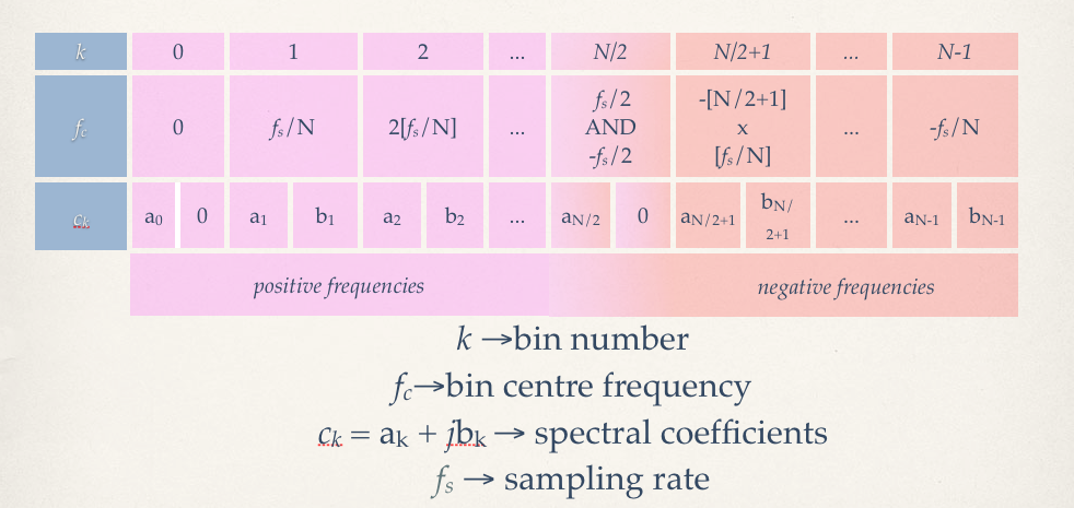
Why stop at half the sampling rate, 22.05 kHz (aka the Nyquist frequency)? Well, because this is the limit for discrete-time signals. The next question is, how many spectral coefficients do we have ? If we started with N discrete time-points, we will have N discrete frequency points. But the points listed above only make up 2206 coefficients, where are the other 2204? Beyond the Nyquist frequency we fold back to the negative spectrum and continue incrementing. So the following points will be -22040, -22030, ..., -20, -10. The halfway point actually represents both the positive and the negative Nyquist frequency (fig.2).

Clearly, the DFT is not the FT, so we do not get the same fine-grained detail in frequencies that we would perhaps have liked. However, there is plenty of good information about the spectrum which can be used in various applications. One important point that should be made at this point is that the DFT decomposes the signal being analysed in N components, which are multiples of the fundamental analysis frequency. This guarantees that if we add these N components together, we will get the back the original signal. The analysis might not be too meaningful, but it still correct. In the special case where we have a periodic signal, where a full period of a waveform is captured by the analysis window, we will be able to recuperate the exact frequencies, amplitudes and phases of that signal (as shown in fig.1).

Another way at looking at the DFT results is to think of each frequency point as the centre of an analysis band, and the magnitude of its coefficient as the amount of energy in that band. This is how spectral displays often work, plotting the magnitude of these coefficients. A fast algorithm for calculating the DFT is normally used, the Fast Fourier Transform (FFT), so operations of spectral analysis can be very computationally efficient.

The Phase Vocoder
The limitations of the raw DFT make it difficult to use in a flexible way for general-purpose audio signal processing. However, it forms the basis for a more useful method of spectral analysis, the Phase Vocoder (PV). We will try to demonstrate how this technique can be seen as an enhancement to DFT analysis.

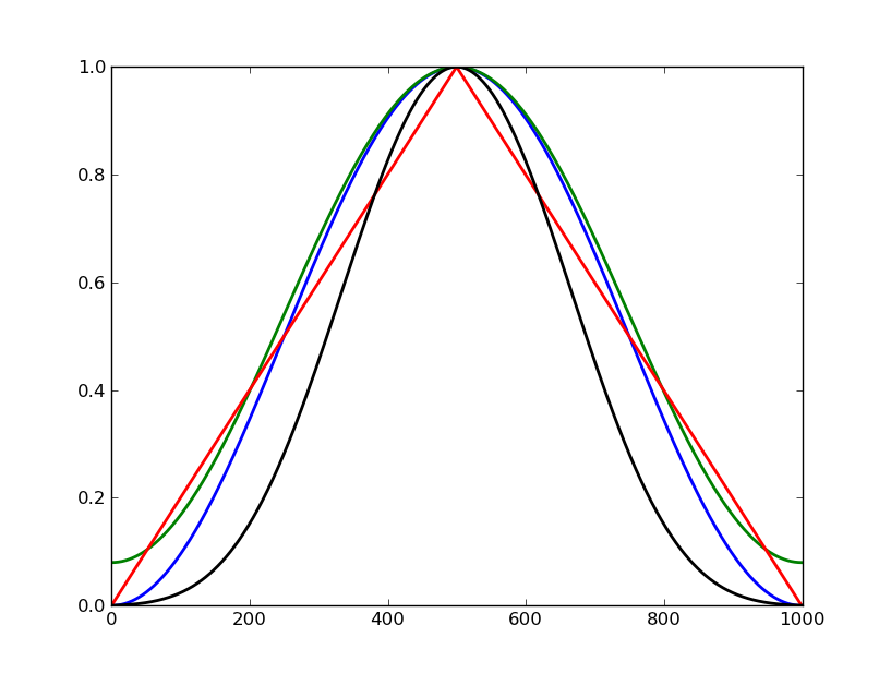
The first step towards the PV is the use of smoothing envelopes to shape the analysis signal, so that we eliminate any harsh cuts or discontinuities at its ends (where the signal was cut for the DFT operation). These envelopes are also known as analysis windows (the case we have used before is the rectangular window, which just extracts the audio block, without any smoothing). The net effect of this is to reduce artefacts, that is, spurious information that the DFT process has generated. Commonly-used windows are the inverse-raised cosine ones, such as the Von Hann (also known as Hanning) and Hamming. These and other window shapes are shown in fig.3.

Secondly, we need to make the operation time-varying. Originally, the DFT was a single-shot analysis, the ‘picture’ of the spectrum at a given time. Now we want to make it so that we have a dynamic analysis of the sound as it changes through time. To do this, we have to take a sequence of windows, which can be, minimally spaced by one sampling period, but generally taken a larger time interval. The space between the analysis frames is known as the hopsize. Generally speaking, the largest practical hopsize used is a quarter of a window length. Now we have a series of spectral analyses, frames, containing N coefficients each, ordered in time.

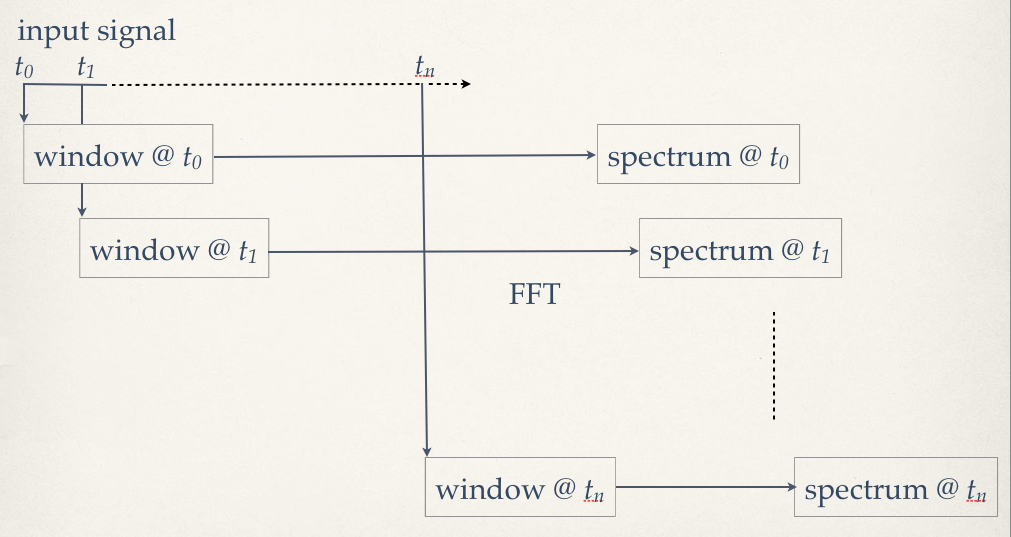
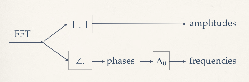
With these modifications (windowing and time-varying analysis, fig.4), we can start to define the Phase Vocoder analysis. The principle is this: for every DFT frequency point, which we will now call a frequency bin, we will be able to obtain time-varying frequency and amplitude data. The latter is simply obtained by calculating the magnitude of each coefficient. The frequency data is extracted by first taking the phases of coefficients, then bin by bin, finding the phase differences between consecutive frames. The phase difference is going to be equivalent to the frequency detected at that bin: how much the sinusoid has ‘moved’ between analysis snapshots (fig.4).

For the resynthesis of PV data we can use straightforward additive synthesis, since we have frequencies and amplitudes, we can drive a bank of sinusoidal oscillators with this data. Alternatively, and often more efficiently, we can reverse the operations used to obtain the amplitude and frequency data from the spectral coefficients and apply the Inverse Discrete Fourier Transform (using the FFT algorithm) to recreate each analysis frame. If the frequencies are in Hz, they are converted to radians per hopsize, then integrated (ie. added) to get the current phase. These, together with the amplitude are then converted into the complex form of the coefficients. The analysis window is then reapplied to each frame and we overlap-add them in sequence to produce the output waveform.

The advantage of the PV representation is that now we have more meaningful analysis data, instead of a block of coefficients, we have time-varying amplitudes and frequencies on each bin. This is much more amenable to further manipulation than raw spectral data. For instance, we can perform time scaling (contraction, stretching) that is independent of frequency.